Телефон: 8-800-350-22-65
Напишите нам:
MAX:
WhatsApp:
Telegram:
Прием заявок круглосуточно
График работы офиса: с 9:00 до 23:00 Нск (с 5:00 до 19:00 Мск)

Статья опубликована в рамках: CIII Международной научно-практической конференции «Вопросы технических и физико-математических наук в свете современных исследований» (Россия, г. Новосибирск, 23 сентября 2026 г.)

Наука: Математика

Секция: Математическая физика

Скачать книгу(-и): Скачать книгу

Библиографическое описание:
Tran D.T. NONLINEAR SURFACE WAVES IN A VISCOUS FLUID LAYER // Вопросы технических и физико-математических наук в свете современных исследований: сб. ст. по матер. CIII междунар. науч.-практ. конф. № 9(94). – Новосибирск: СибАК, 2026. – С. 96-108.
Проголосовать за статью
Дипломы участников
У данной статьи нет
дипломов

NONLINEAR SURFACE WAVES IN A VISCOUS FLUID LAYER

Tran Dinh Tuong

teacher, University of Finance-Marketing, Viet Nam, Hồ Chí Minh

Abstract

This paper investigates the nonlinear propagation of the waves on the free surface of an infinitely deep, viscous, and incompressible fluid layer. Utilizing the first Stokes method, the governing equations are solved with second-order approximation accuracy. The study successfully derives analytical expressions for the trajectories of fluid particles and the velocity of the near-surface current. Furthermore, the comprehensive analysis demonstrates how fluid viscosity and depth systematically modulate both the transport velocity and the specific geometry of particle orbital motions.

Аннотация

В данной работе исследуется нелинейное распространение волн на свободной поверхности бесконечно глубокого, вязкого и несжимаемого слоя жидкости. С использованием первого метода Стокса решаются определяющие уравнения с точностью второго порядка аппроксимации. В работе успешно получены аналитические выражения для траекторий частиц жидкости и скорости приповерхностного течения. Кроме того, всесторонний анализ демонстрирует, как вязкость жидкости и глубина систематически модулируют как скорость переноса, так и конкретную геометрию орбитальных движений частиц.

Keywords: Nonlinear surface waves; viscous fluid dynamics; fluid particle trajectories; Stokes expansion method; near-surface current velocity.

Ключевые слова: Нелинейные поверхностные волны; динамика вязкой жидкости; траектории частиц жидкости; метод разложения Стокса; скорость приповерхностного течения.

1. Introduction

The study of surface wave propagation within fluid layers is a fundamental pillar of modern fluid dynamics, with expansive applications ranging from ocean engineering to industrial coating processes. Over the past several decades, mathematical modeling of these phenomena has advanced significantly. Initial breakthrough formulations focused on the behavior of waves within ideal, inviscid fluids, as thoroughly detailed in the seminal works of Sretenskii [1] and Aleshkov [2]. In particular, Aleshkov successfully identified the nonlinear trajectories of liquid particles under idealized conditions [2]. While the assumption of an ideal fluid simplifies the underlying governing equations, it fails to account for the energy dissipation mechanisms inherently present in real-world fluids due to internal friction.

To bridge this gap, substantial research has been dedicated to incorporating viscosity into wave dynamics models. The exact linear solutions for viscous fluids have been extensively documented in classic hydrodynamic literature [3, 4] and updated by Barinov [5]. However, real-world wave phenomena are inherently nonlinear, characterized by high amplitudes where linear approximations lose physical validity. Resolving the fully nonlinear boundary value problem for a viscous fluid layer presents severe mathematical challenges due to the tight coupling between the free moving boundary and viscous shear stresses. Consequently, prior successful attempts at nonlinear modeling have been strictly limited to the approximation of low-viscosity (weakly viscous) fluids, such as the asymptotic formulations developed by Barinov and Basinsky [6]. More recently, advanced formulations have begun to address time-dependent nonlinear gravity–capillary surface waves by deeply analyzing the intricate balance between viscous dissipation and wind forcing mechanisms [7].

A comprehensive mathematical treatment that simultaneously addresses high viscosity, arbitrary depth considerations, and full second-order nonlinear geometric effects remains underdeveloped. Furthermore, while recent frameworks have explored how surface waves interact with sheared currents to induce distinct Stokes drift patterns [8], a localized analysis for a purely viscous layer requires explicit geometric validation. This paper aims to fill these critical gaps in the literature. We establish a rigorous nonlinear formulation for wave movement on the free surface of an incompressible viscous fluid layer of infinite depth. By deploying the first Stokes parameter expansion method up to the second-order approximation, we derive explicit analytical expressions for fluid velocity components, dynamic pressure fields, and the exact geometric evolution of the free boundary. Ultimately, this study offers a detailed analysis of how internal fluid viscosity and spatial depth systematically modulate the Stokes drift velocity and the structural deformation of fluid particle orbital trajectories.

2. Materials and Methods

2.1. Nonlinear Problem of Waves on a Viscous Fluid Surface

An infinitely deep layer of a viscous incompressible fluid is considered. The free surface of the layer borders a medium of negligibly density, characterized by a constant pressure P_{a} (in particular, atmospheric pressure). A Cartesian coordinate system is defined such that the plane z^{*} = 0 coincides with the undisturbed surface, and the z^{*} - axis is directed opposite to the gravity vector g . The motion of the fluid occurs in the x^{*}z^{*} plane with a velocity f^{*} = \left( f^{*}\left( t^{*},x^{*},z^{*} \right),0,v^{*}\left( t^{*},x^{*},z^{*} \right) \right) . Asterisks, where necessary, denote physical (dimensional) quantities. Let a wave of length \lambda propagate in the positive direction of the \mathrm{x}^{\mathrm{*}}\mathrm{\ } - axis. The wavelength is much greater than its height \left( \lambda \gg \xi_{\text{max~}}^{*} \right) . In the region occupied by the fluid, the equations of continuity and motion are satisfied:

divf^{*} = 0,\ \frac{\partial f^{*}}{\partial t^{*}} + \left( f^{*}\nabla \right)f^{*} = - \frac{1}{\rho}\nabla p^{*} + \frac{\mu}{\rho}\Delta f^{*}, (1)

Here, p^{*} = P - P_{a} + \rho.g.z^{*}\ is the dynamic pressure, \rho is the density, P is the pressure, and \mu is the dynamic viscosity coefficient. On the free surface z^{*} = \xi^{*}\left( t^{*},x^{*} \right) , the kinematic and dynamic conditions are specified as:

v^{*}\ = \frac{\partial\xi^{*}}{\partial t^{*}} + f^{*}\frac{\partial\xi^{*}}{\partial x^{*}},\ \ p_{nn}\ = - P_{a},\ p_{n\tau} = 0. (2)

At infinite depth, the fluid velocity must decay, i.e., the following condition is satisfied:

f^{*} \rightarrow 0,z^{*} \rightarrow - \infty. (3)

The system of equations (1) and boundary conditions (2), (3) is closed and constitutes a nonlinear boundary value problem for determining the characteristics of wave motion. Let us introduce the following dimensionless variables and quantities:

\begin{matrix} f^{*} = \varepsilon c_{0}f,\nu_{0} = \frac{\mu k}{\rho c_{0}},\ p^{*} = \varepsilon\rho c_{0}^{2}p,\ x = kx^{*},\xi^{*} = \varepsilon\frac{\xi}{k},\ \\ t = kct^{*},\ \ z = kz^{*},\ \alpha = \frac{c}{c_{0}} = \frac{\omega}{\omega_{0}},\ c_{0}^{2} = \frac{g}{k}, \\ \end{matrix}

where c_{0} and \omega_{0} are, respectively, the phase velocity and wave frequency of the linear problem for an ideal fluid; c and \omega are the phase velocity and wave frequency; \varepsilon = k\xi_{\text{max~}}^{*} is the small wave parameter; and k = 2\pi/\lambda is the wave number.

In dimensionless variables, problem (1) – (3) takes the form:

Divf = 0,\ \alpha\frac{\partial f}{\partial t} - \nu_{0}\Delta f + \nabla p = - \varepsilon(f\nabla)f,\ \ v - \alpha\frac{\partial\xi}{\partial t} = \varepsilon f\frac{\partial\xi}{\partial x},\ z = \varepsilon\xi,

p - \xi - 2\nu_{0}\frac{\partial v}{\partial z} = - \varepsilon\nu_{0}\left( \frac{\partial f}{\partial z} + \frac{\partial v}{\partial x} \right)\frac{\partial\xi}{\partial x} + \varepsilon^{2}\left( \frac{\partial\xi}{\partial x} \right)^{2}\left( \xi - p - 2\nu_{0}\frac{\partial v}{\partial z} \right),\ z = \varepsilon\xi, (4)

\nu_{0}\left( \frac{\partial f}{\partial z} + \frac{\partial v}{\partial x} \right)\left( 1 - \varepsilon^{2}\left( \frac{\partial\xi}{\partial x} \right)^{2} \right) = - 4\nu_{0}\frac{\partial v}{\partial z}\frac{\partial\xi}{\partial x},\ z = \varepsilon\xi, f \rightarrow 0,\ z \rightarrow - \infty.

Due to the smallness of the wave parameter \varepsilon , the boundary conditions on the free surface z = \varepsilon\xi are reduced to conditions on the fixed surface z = 0 by expanding the constituent functions into a Maclaurin series. We seek the solution to the problem in the form of series in terms of the parameter \varepsilon :

f = \sum_{i = 1}^{\infty}\varepsilon^{i - 1}f_{i};\ \ f_{n} = \left( f_{i},0,v_{i} \right);\ \ \ \xi = \sum_{i = 1}^{\infty}\varepsilon^{i - 1}\xi_{i};\ \ p = \sum_{i = 1}^{\infty}\varepsilon^{i - 1}p_{i}.

Substituting these series into equations (4) and into the boundary conditions expanded in the neighborhood of zero, and equating the coefficients of identical powers of \varepsilon , we obtain the problems in the first two approximations.

In the first approximation, the problem takes the form: at \varepsilon^{0}

divf_{1} = 0,\ \alpha\frac{\partial f_{1}}{\partial t} - \nu_{0}\Delta f_{1} = - \nabla p_{1},\ v_{1} = \alpha\frac{\partial\xi_{1}}{\partial t},

p_{1} - \xi_{1} - 2\nu_{0}\frac{\partial v_{1}}{\partial z} = 0,\ \frac{\partial f_{1}}{\partial z} + \frac{\partial v_{1}}{\partial x} = 0,\ z = 0,f_{1} \rightarrow 0,z \rightarrow - \infty. (5)

For the second approximation: at \varepsilon^{1}

divf_{2} = 0,\ \alpha\frac{\partial f_{2}}{\partial t} - \nu_{0}\Delta f_{2} = - \nabla p_{2} - \left( f_{1}\nabla \right)f_{1};

v_{2} = \alpha\frac{\partial\xi_{2}}{\partial t} + \frac{\partial}{\partial x}\left( f_{1}\xi_{1} \right),p_{2} - \xi_{2} - 2\nu_{0}\frac{\partial v_{2}}{\partial z} = \xi_{1}\frac{\partial}{\partial z}\left( 2\nu_{0}\frac{\partial v_{1}}{\partial z} - p_{1} \right),\ z = 0; (6)

\frac{\partial f_{2}}{\partial z} + \frac{\partial v_{2}}{\partial x} = 4\frac{\partial f_{1}}{\partial x}\frac{\partial\xi_{1}}{\partial x} - \xi_{1}\frac{\partial}{\partial z}\left( \frac{\partial f_{1}}{\partial z} + \frac{\partial v_{1}}{\partial x} \right),\ z = 0; f_{2} \rightarrow 0,z \rightarrow - \infty.

The solution to the linear problem (5) has the form [5]:

f_{1} = Ae^{- \frac{\beta}{\alpha}t}\left\lbrack \left( aE_{1} + bE_{2} \right)\cos(x - t) + e^{z}\cos(x - t) + \left( aE_{2} - bE_{1} \right)sin(x - t) \right\rbrack;

v_{1} = Ae^{- \frac{\beta}{\alpha}t}\left\{ {E_{1}\cos(x - t) + e}^{z}\sin(x - t) + E_{2}sin(x - t) \right\};

p_{1} = Ae^{z - \frac{\beta}{\alpha}t}\left( \alpha\cos(x - t) + \beta\sin(x - t) \right);\ \ (7)

\xi_{1} = \frac{A}{\alpha^{2} + s^{2}}e^{- \frac{\beta}{\alpha}t}\left( \alpha\cos(x - t) + s\sin(x - t) \right);

E_{1}(z) = e^{bz}\left( B_{1}\cos{az} - B_{2}\sin{az} \right);\ E_{2}(z) = e^{bz}\left( B_{2}\cos{az} + B_{1}\sin{az} \right) ;

B_{1} = - \frac{2\nu_{0}\alpha A}{\left( \alpha^{2} + s^{2} \right)};\ B_{2} = - \frac{2\nu_{0}sA}{\left( \alpha^{2} + s^{2} \right)}.

Here, \beta is the dimensionless damping decrement ( \beta\omega_{0}\ is the dimensional one), A is the amplitude parameter, and s = 2\nu_{0} - \beta . The parameters a and b are related by the following expressions: a^{2} = b^{2} - 1 + \beta/\nu_{0} and 2ab = \alpha/\nu_{0} .

The wave frequency is expressed through the damping decrement as follows:

\alpha^{2} = 1 + s^{2} - 4\nu_{0}^{3}/s.

For the damping decrement itself, the following equation is obtained:
s^{6} + s^{4} - 4\nu_{0}^{4}s^{2} - 4\nu_{0}^{6} = 0 , the analytical solution of which has been found but is not presented here due to its cumbersomeness.

Substituting expressions (7) into problem (6), we obtain a system of linear inhomogeneous equations and boundary conditions for determining the unknown functions f_{2},v_{2},p_{2} , and \xi_{2} , the solution of which has the form:

f_{2} = e^{- \frac{2\beta}{\alpha}t}\left( \left\{ e^{2z}D_{2} + 1/2\left\lbrack a_{1}E_{3} + b_{1}E_{4} + aE_{5} + (b + 1)E_{6} \right\rbrack \right\} cos(2x - 2t) + \right.\

\left. \ \left\{ - e^{2z}D_{1} + 1/2\left\lbrack a_{1}E_{4} - b_{1}E_{3} + aE_{6} - (b + 1)E_{5} \right\rbrack \right\} sin(2x - 2t) \right);

v_{2} = e^{- \frac{2\beta}{\alpha}t}\left\lbrack \left( e^{2z}D_{1} + E_{3} + E_{5} \right)cos(2x - 2t) + \left( e^{2z}D_{2} + E_{4} + E_{6} \right)sin(2x - 2t) \right\rbrack;

p_{2} = e^{- \frac{2\beta}{\alpha}t}\left\{ \left\lbrack e^{2z}\left( \beta D_{1} + \alpha D_{2} \right) + E_{7} \right\rbrack cos(2x - 2t) + \left\lbrack e^{2z}\left( \beta D_{2} - \alpha D_{1} \right) + E_{8} \right\rbrack \times \right.\

sin(2x - 2t) - e^{z}AE_{2} + AB_{2} + A^{2}\left\lbrack \left( 2\nu_{0} - \beta s \right)/\left( \alpha^{2} + s^{2} \right) - e^{2z} \right\rbrack/2 +

\left. \ \left( B_{1}^{2} + B_{2}^{2} \right)\left( 1 - e^{2z} \right)/2 \right\} ;

\xi_{2} = \frac{e^{- \frac{2\beta}{\alpha}t}}{2\left( \alpha^{2} + \beta^{2} \right)}\left\{ \left\lbrack \alpha\left( {B_{4} + D}_{2} - Q_{2}K_{2} \right) - \beta\left( {B_{3} + D}_{1} + Q_{1} + K_{1} \right) \right\rbrack \times \right.\

cos(2x - 2t) - \left\lbrack \beta\left( {B_{4} + D}_{2} - Q_{2} + K_{2} \right) + \alpha\left( {B_{3} + D}_{1} + Q_{1} + K_{1} \right) \right\rbrack \times

sin(2x - 2t)\},

Where E_{3}(z) = e^{b_{1}z}\left( - B_{4}\sin{{(a}_{1}z)} + B_{3}\cos{{(a}_{1}z)} \right);

E_{4}(z) = e^{b_{1}z}\left( B_{4}cos{(a}_{1}z) + B_{3}sin{(a}_{1}z \right) ;

E_{5}(z) = e^{(b + 1)z}\left( K_{1}\cos{(az)} - K_{2}\sin{(az)} \right);

E_{6}(z) = e^{(b + 1)z}\left( K_{2}\cos(az) + K_{1}\sin(az) \right) ;

E_{7}(z) = e^{(b + 1)z}\left( G_{1}\cos(az) - G_{2}\sin(az) \right);

E_{8}(z) = e^{(b + 1)z}\left( G_{2}\cos(az) + G_{1}\sin(az) \right);\ a_{1}^{2} = b_{1}^{2} - 4 + \frac{2\beta}{\nu_{0}};\ a_{1}b_{1} = \frac{\alpha}{\nu_{0}};

\ K_{1} = \frac{\left\{ \left\lbrack aR_{2} + (b + 1)R_{1} \right\rbrack C_{1} - \left\lbrack - (b + 1)R_{2} + aR_{1} \right\rbrack C_{2} \right\}}{\Delta_{1}};\ K_{2} = \frac{\left\{ \left\lbrack aR_{1} - (b + 1)R_{2} \right\rbrack M_{1} + \left\lbrack (b + 1)R_{1} + aR_{2} \right\rbrack M_{2} \right\}}{\Delta_{1}};

G_{1} = \frac{\left\{ \left\lbrack \alpha a + \beta(b - 1) \right\rbrack K_{1} + 2R_{2} - \left\lbrack \alpha(1 - b) + \beta a \right\rbrack K_{2} \right\}}{4};\ \

G_{2} = \frac{\left\{ \left\lbrack \alpha(1 - b) + \beta a \right\rbrack K_{1} + 2R_{1} + \left\lbrack \alpha a + \beta(b - 1) \right\rbrack K_{2} \right\}}{4}\Delta_{1} = \frac{\left( M_{1}^{2} + M_{2}^{2} \right)}{2} ;

\begin{matrix} M_{1} = \frac{\left\lbrack - \alpha\left( \beta + 2\nu_{0} \right) + 4a\nu_{0}^{2} \right\rbrack}{\left( 2\nu_{0} \right)},\ M_{2} = \frac{\left\lbrack 8b\nu_{0}^{2} + \beta_{0}^{2} - 4\nu_{0}s - \alpha_{0}^{2} \right\rbrack}{\left( 4\nu_{0} \right)}, \\ R_{1} = A\left\lbrack \left( \alpha - 2a\nu_{0} \right)B_{2} + \left( 2b\nu_{0} - s \right)B_{1} \right\rbrack/\left( 2\nu_{0} \right), \\ R_{2} = A\left\lbrack - \left( 2b\nu_{0} - s \right)B_{2} + \left( \alpha - 2a\nu_{0} \right)B_{1} \right\rbrack/\left( 2\nu_{0} \right), \\ \end{matrix}

\begin{matrix} B_{3} = \nu_{0}\left\lbrack s_{1}\left( L_{2} - 4D_{1} \right) + \alpha\left( L_{1} - 4D_{2} \right) \right\rbrack/\Delta_{2},\ \Delta_{2} = s_{1}^{2} + \alpha^{2}, \\ B_{4} = \nu_{0}\left\lbrack s_{1}\left( L_{1} - 4D_{2} \right) - \alpha\left( L_{2} - 4D_{1} \right) \right\rbrack/\Delta_{2},\ s_{1} = 4\nu_{0} - \beta, \\ \end{matrix}

\begin{matrix} L_{1} = A^{2}\left\{ a\left\lbrack 4\nu_{0}^{2}\left( \alpha^{2} - s^{2} \right)/\Delta_{3} - s - K_{1} \right\rbrack + \alpha b\left\lbrack 1 - K_{2} + 8\nu_{0}s/\Delta_{3} \right\rbrack - \right.\ \\ 3\alpha + \left. \ \left\lbrack \left( \beta - 6\nu_{0} \right)K_{2} - \alpha K_{1} \right\rbrack/\left( 2\nu_{0} \right) \right\}/\Delta_{3},\ \Delta_{3} = s^{2} + \alpha^{2} \\ L_{2} = A^{2}\left\{ b\left\lbrack 4\nu_{0}^{2}\left( \alpha^{2} - s^{2} \right)/\Delta_{3} - s - K_{1} \right\rbrack - \alpha a\left\lbrack 1 - K_{2} + 8\nu_{0}s/\Delta_{3} \right\rbrack + \right.\ \\ 3s + \left. \ \left\lbrack \left( \beta - 6\nu_{0} \right)K_{1} + \alpha K_{2} \right\rbrack/\left( 2\nu_{0} \right) \right\}/\Delta_{3}, \\ \end{matrix}

\begin{matrix} D_{1} = \left( F_{1}J_{1} + F_{2}J_{2} \right)/\Delta_{4},\ D_{2} = \left( F_{1}J_{2} - F_{2}J_{1} \right)/\Delta_{4},\ \Delta_{4} = J_{1}^{2} + J_{1}^{2} \\ J_{1} = \left\lbrack 8\nu_{0}^{2}\left( \alpha a_{1} + s_{1}b_{1} \right) - s_{1}/\Delta_{2} \right\rbrack - s_{1},\ J_{2} = \left\lbrack 8\nu_{0}^{2}\left( \alpha b_{1} - s_{1}a_{1} \right) - \alpha/\Delta_{2} \right\rbrack + \alpha, \\ F_{1} = A^{2}\left\lbrack 2\nu_{0}(\alpha - s)/\Delta_{3} + 1 \right\rbrack\left\lbrack 2\nu_{0}(\alpha + s)/\Delta_{3} - 1 \right\rbrack/2 - G_{1} + H_{1}L_{1} + \\ I_{1}K_{1} + I_{2}K_{2} + H_{2}L_{2} + \left( \beta Q_{1} - \alpha Q_{2} \right)/\left( 2\Delta_{5} \right),\ \Delta_{5} = \left( \alpha^{2} + \beta^{2} \right), \\ \end{matrix}

\begin{matrix} F_{2} = 2\alpha\nu_{0}A^{2}\left( 1 - 2s\nu_{0}/\Delta_{3} \right)/\Delta_{3} + I_{2}K_{1} - I_{1}K_{2} + G_{2} - H_{2}L_{1} + H_{1}L_{2} + \\ \frac{\left( \beta Q_{2} + \alpha Q_{1} \right)}{\left( 2\Delta_{5} \right)}, \\ I_{1} = 2b\nu_{0} + \left( 4\nu_{0} - \beta/\Delta_{5} \right)/2,\ I_{2} = - 2a\nu_{0} + \alpha/\left( 2\Delta_{5} \right), \\ H_{1} = \left\lbrack 2\alpha\nu_{0}^{2}b_{1} - 2s_{1}\nu_{0}^{2}a_{1} + \alpha\nu_{0}^{2}s/\Delta_{5} \right\rbrack/\Delta_{3}, \\ H_{2} = \left\lbrack 2\alpha\nu_{0}^{2}a_{1} + 2s_{1}\nu_{0}^{2}b_{1} + \left( \beta s_{1} - \alpha^{2} \right)/\Delta_{5} \right\rbrack/\Delta_{3}. \\ \end{matrix}

2.2. Wave Trajectories of Fluid Particles

The physical coordinates of the particle z^{*}\left( t^{*} \right),\ x^{*}\left( t^{*} \right) satisfy the equations:

\ \frac{dz^{*}}{dt^{*}} = v^{*},\ \frac{dx^{*}}{dt^{*}} = f^{*}.

The physical time must be made dimensionless using the oscillation frequency of the fluid particle \sigma , since for nonlinear waves, even in an ideal fluid, \sigma does not coincide with the wave frequency.

Given that: z^{*} = \frac{z}{k},\ x^{*} = ct^{*} + \frac{x}{k},\ \ f^{*} = \varepsilon c_{0}f,t^{*} = t/\sigma, the equations describing the particle motion in the wave can be represented in the form:

\frac{dx}{dt} = \varepsilon\left( \frac{t}{\alpha} \cdot \frac{ck}{\sigma} \right)^{'}f - \left( t \cdot \frac{ck}{\sigma} \right)^{'},\ \frac{dz}{dt} = \varepsilon\left( \frac{t}{\alpha} \cdot \frac{ck}{\sigma} \right)^{'}v. (8)

Let us set:

x = \sum_{i = 0}^{\infty}\mspace{2mu}\varepsilon^{i}x_{i},\ z = \sum_{i = 0}^{\infty}\mspace{2mu}\varepsilon^{i}z_{i},\ \frac{kc}{\sigma} = 1 + \sum_{i = 1}^{\infty}\mspace{2mu}\varepsilon^{i}\gamma_{i}. (9)

Substituting series (9) and the expressions for the velocity components into the equations of motion (8), we obtain the following equations for determining the first three coefficients: \frac{dx_{0}}{dt} = - 1,\ \frac{dz_{0}}{dt} = 0 ,

\begin{matrix} \frac{dx_{1}}{dt} = & \frac{A}{\alpha}e^{- \frac{\beta}{\alpha}t}\left\{ \left\lbrack e^{z_{0}} + aE_{1}\left( z_{0} \right) + bE_{2}\left( z_{0} \right) \right\rbrack cosx_{0} + \left\lbrack aE_{2}\left( z_{0} \right) - bE_{1}\left( z_{0} \right) \right\rbrack sinx_{0} \right\} - \\ & \ \left( t\gamma_{1} \right)^{'},\ \frac{dz_{1}}{dt} = \frac{A}{\alpha}e^{- \frac{\beta}{\alpha}t}\left\{ \left\lbrack e^{z_{0}} + E_{1}\left( z_{0} \right) \right\rbrack\cos x_{0} + E_{2}\left( z_{0} \right)\sin x_{0} \right\}, \\ \end{matrix}

\begin{matrix} & \frac{dx_{2}}{dt} = \frac{e^{- \frac{2\beta}{\alpha}t}}{\alpha}\left( \left\{ e^{2z_{0}}D_{2} + 1/2\left\lbrack a_{1}E_{3}\left( z_{0} \right) + b_{1}E_{4}\left( z_{0} \right) + aE_{5}\left( z_{0} \right) + (b + 1)E_{6}\left( z_{0} \right) \right\rbrack \right\} \times \right.\ \\ & \ cos2x_{0} + \left\{ - e^{2z_{0}}D_{1} + 1/2\left\lbrack a_{1}E_{4}\left( z_{0} \right) - b_{1}E_{3}\left( z_{0} \right) + aE_{6}\left( z_{0} \right) - (b + 1)E_{5}\left( z_{0} \right) \right\rbrack \right\} \times \\ \end{matrix}

\begin{matrix} & \left. \ sin2x_{0} \right) - \left( t\gamma_{2} \right)^{'} + \frac{e^{- \frac{\beta}{\alpha}t}}{\alpha}\left( \left\{ Az_{1}e^{z_{0}} + b\left( 2az_{1} - x_{1} \right)E_{1}\left( z_{0} \right) - \left\lbrack \left( a^{2} - b^{2} \right)z_{1} - ax_{1} \right\rbrack \times \right.\ \right.\ \\ & \left. \ E_{2}\left( z_{0} \right) \right\} cosx_{0} + \left\{ - Ax_{1}e^{z_{0}} + b\left( 2az_{1} - x_{1} \right)E_{2}\left( z_{0} \right) + \left\lbrack \left( a^{2} - b^{2} \right)z_{1} - ax_{1} \right\rbrack \times \right.\ \\ \end{matrix}

\left. \ \left. \ E_{1}\left( z_{0} \right) \right\} sinx_{0} \right),

\begin{matrix} \frac{dz_{2}}{dt} = & \frac{e^{- \frac{2\beta}{\alpha}t}}{\alpha}\left\lbrack \left( e^{2z_{0}}D_{1} + E_{3}\left( z_{0} \right) + E_{5}\left( z_{0} \right) \right)cos2x_{0} + \left( e^{2z_{0}}D_{2} + E_{4}\left( z_{0} \right) + E_{6}\left( z_{0} \right) \right) \times \right.\ \\ & \left. \ sin2x_{0} \right\rbrack + \frac{e^{- \frac{\beta}{\alpha}}t}{\alpha}\left\{ \left\lbrack Ax_{1}e^{z_{0}} + bz_{1}E_{1}\left( z_{0} \right) + \left( x_{1} - az_{1} \right)E_{2}\left( z_{0} \right) \right\rbrack cosx_{0} + \right.\ \\ & \left. \ \left\lbrack Az_{1}e^{z_{0}} + bz_{1}E_{2}\left( z_{0} \right) - \left( x_{1} - az_{1} \right)E_{1}\left( z_{0} \right) \right\rbrack sinx_{0} \right\}. \\ \end{matrix}

Solving these equations sequentially, we obtain the following expressions:

x_{0} = x_{L} - t,\ z_{0} = z_{L},\ \gamma_{1} = 0;

x_{1} = \frac{e^{- \frac{\beta}{\alpha}t}}{\Delta_{5}}\left\{ \left\lbrack - \beta Ae^{z_{L}} - (\alpha b + \beta a)E_{1}\left( z_{L} \right) + (\alpha a - \beta b)E_{2}\left( z_{L} \right) \right\rbrack cos\left( x_{L} - t \right) + \right.\

\left. \ \left\lbrack - \alpha Ae^{z_{L}} - (\alpha b + \beta a)E_{2}\left( z_{L} \right) - (\alpha a - \beta b)E_{1}\left( z_{L} \right) \right\rbrack sin\left( x_{L} - t \right) \right\};

z_{1} = \frac{e^{- \frac{\beta}{\alpha}t}}{\Delta_{5}}\left\lbrack \left( \alpha Ae^{z_{L}} - \beta E_{1}\left( z_{L} \right) + \alpha E_{2}\left( z_{L} \right) \right)cos\left( x_{L} - t \right) + \right.\

\left( - \beta Ae^{z_{L}} - \beta E_{2}\left( z_{L} \right) - \alpha E_{1}\left( z_{L} \right) \right)\sin\left( x_{L} - t \right);

x_{2} = \frac{e^{- \frac{2\beta}{\alpha}t}}{2\Delta_{5}}\left( \left\{ - \left( \alpha D_{1} + \beta D_{2} \right)e^{2z_{L}} - \left( \beta a_{1} + \alpha b_{1} \right)E_{3}\left( z_{L} \right)/2 + \left( \alpha a_{1} - \beta b_{1} \right) \times \right.\ \right.\

E_{4}\left( z_{L} \right)/2 + Ae^{z_{L}}\left\lbrack \left( - \beta^{2}b + 2\alpha\beta a + \alpha^{2}b \right)/\Delta_{5} + \left( \alpha^{2} - \beta^{2} \right)/\Delta_{5} - \beta/\left( 2\nu_{0} \right) \right\rbrack \times

E_{1}\left( z_{L} \right) + Ae^{z_{L}}\left\lbrack \left( 2\alpha\beta b + \beta^{2}a - \alpha^{2}a \right)/\Delta_{5} - 2\alpha\beta/\Delta_{5} + \alpha/\left( 2\nu_{0} \right) \right\rbrack E_{2}\left( z_{L} \right) -

\left. \ \lbrack\alpha(b + 1) + \beta a\rbrack E_{5}\left( z_{L} \right)/2 + \lbrack\alpha a - \beta(b + 1)\rbrack E_{6}\left( z_{L} \right)/2 \right\}\cos\left( 2x_{L} - t \right) -

\left( \alpha a_{1} - \beta b_{1} \right)E_{3}\left( z_{L} \right) + \left\{ \left( \beta D_{1} - \alpha D_{1} \right)e^{2z_{L}} - \left( \beta a_{1} + \alpha b_{1} \right)E_{4}\left( z_{L} \right) + \right.\

Ae^{z_{L}}\left\lbrack \left( 2\alpha\beta a - \beta^{2}b + \alpha^{2}b \right)/\Delta_{5} + \left( \alpha^{2} - \beta^{2} \right)/\Delta_{5} - \beta/\left( 2\nu_{0} \right) \right\rbrack E_{2}\left( z_{L} \right) -

Ae^{z_{L}}\left\lbrack \frac{\left( 2\alpha\beta b - \alpha^{2}a + \beta^{2}a \right)}{\Delta_{5}} + \frac{\alpha}{\left( 2\nu_{0} \right)} - \frac{2\alpha\beta}{\Delta_{5}} \right\rbrack E_{1}\left( z_{L} \right) -

\left. \ \lbrack\alpha(b + 1) + \beta a\rbrack E_{6}\left( z_{L} \right)/2 - \lbrack\alpha a - \beta(b + 1)\rbrack E_{5}\left( z_{L} \right)/2 \right\} sin\left( 2x_{L} - t \right)),

\begin{matrix} z_{2} = \frac{e^{- \frac{2\beta}{\alpha}t}}{2\Delta_{5}}\left\{ \left\lbrack \left( \alpha D_{2} - \beta D_{1} \right)e^{2z_{L}} + \alpha E_{4}\left( z_{L} \right) - \beta E_{3}\left( z_{L} \right) + \alpha E_{6}\left( z_{L} \right) - \beta E_{5}\left( z_{L} \right) \right\rbrack \times \right.\ \\ cos\left( 2x_{L} - 2t \right) + \left\lbrack - \left( \alpha D_{1} + \beta D_{2} \right)e^{2z_{L}} - \alpha E_{3}\left( z_{L} \right) - \beta E_{4}\left( z_{L} \right) - \alpha E_{5}\left( z_{L} \right) - \right.\ \\ \left. \ \beta E_{6}\left( z_{L} \right) \right\rbrack sin\left( 2x_{L} - 2t \right) + Ae^{z_{L}}\left\lbrack aE_{1}\left( z_{L} \right) + (b + 1)E_{2}\left( z_{L} \right) + A^{2} \right\rbrack + \\ \left. \ be^{bz_{L}}\left( B_{1}^{2} + B_{2}^{2} \right) \right\}, \\ \end{matrix}

\begin{matrix} \gamma_{2} = \frac{1 - e^{- \frac{2\beta}{\alpha}t}}{4\beta\nu_{0}\Delta_{5}t}\left\lbrack 2\alpha\nu_{0}A^{2}e^{2z_{L}} + Ae^{z_{L}}\left( \alpha^{2} - \beta^{2} + 2a\alpha\nu_{0} \right)E_{1}\left( z_{L} \right) + 2\alpha Ae^{z_{L}} \times \right.\ \\ \left( \nu_{0} + b\nu_{0} - \beta \right)E_{2} + \alpha e^{2bz_{L}}\left( B_{1}^{2} + B_{1}^{2} \right)\left( 2a^{2}\nu_{0} + 2\nu_{0} - 3\beta \right), \\ \end{matrix}

where x_{L},z_{L} are the Lagrangian coordinates.

The quantity f_{s} = c - \sigma/k represents the transport velocity along the horizontal axis. Its approximate expression has the form:

f_{s} = c\left( 1 - \frac{\sigma}{ck} \right) = c\left( 1 - \frac{1}{1 + \varepsilon^{2}\gamma_{2}} \right) \approx \varepsilon^{2}c\gamma_{2}. (10)
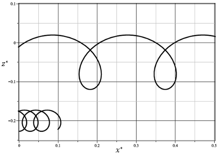
Figure 1. Fluid particle trajectories at \mathrm{\nu}\mathrm{=}\mathrm{10}^{\mathrm{- 6}} {\text{ }\mathrm{m}}^{\mathrm{2}}\mathrm{/s}
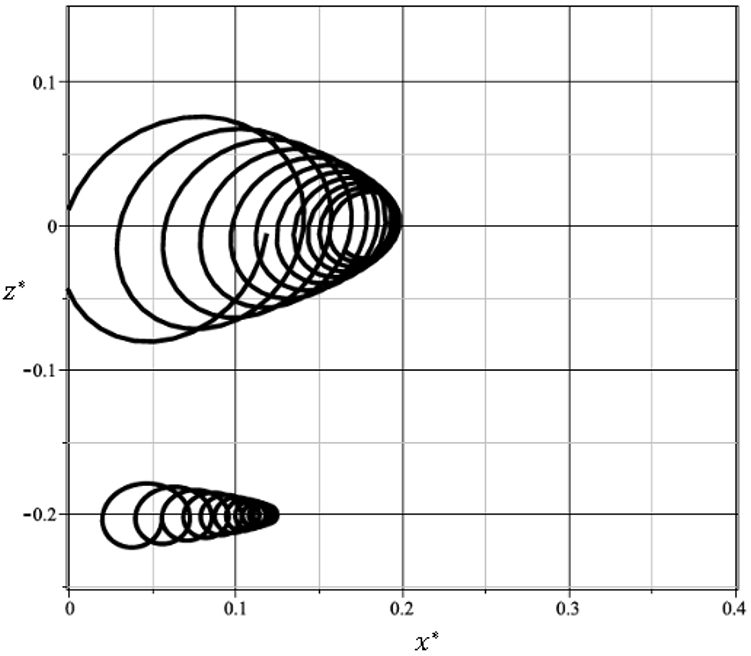
Figure 2. Fluid particle trajectories at \mathrm{\nu}\mathrm{= 2 \bullet}\mathrm{10}^{\mathrm{- 3}} {\text{ }\mathrm{m}}^{\mathrm{2}}\mathrm{/s}

As an example, the motion trajectories of fluid particles are plotted for small (Fig. 1) and large (Fig. 2) values of the kinematic viscosity coefficient. It can be seen that particles near the surface move faster than particles at depth, which is due to the presence of the near-surface Stokes drift current characterized by the transport velocity (10). With an increase in viscosity, both the amplitude of wave disturbances and the transport velocity decay more rapidly. Furthermore, near the surface at high viscosity, the trajectories tilt forward in the direction of motion at their highest point, a phenomenon that is not observed at greater depths. This can be explained by the influence of viscous tangential shear stresses on the free surface.

Thus, an asymptotic solution to the nonlinear problem has been obtained with accuracy up to terms of the second order in the small amplitude parameter. Expressions have been derived for the trajectories of fluid particles, as well as for the velocity of the near-surface Stokes current.

3. Conclusion

This paper successfully establishes a second-order nonlinear asymptotic solution for wave propagation on the free surface of an infinitely deep, viscous, incompressible fluid layer using the first Stokes method. The mathematical framework derives explicit analytical expressions for fluid velocity fields, dynamic pressure, and free surface geometry. The analysis reveals that internal fluid viscosity and depth systematically modulate particle dynamics. Near – surface particles advance faster than deeper particles due to a distinct Stokes drift current, though both wave amplitude and transport velocity decay rapidly as viscosity increases. Furthermore, under high viscosity conditions, tangential shear stresses cause upper-layer particle trajectories to tilt forward at their highest orbital points – a structural deformation absent at greater depths. Ultimately, these derived expressions provide a reliable theoretical foundation for mass transport predictions in viscous fluid layers.

Acknowledgments

This research is funded by University of Finance-Marketing, Viet nam.

References

1. Sretenskii, L.N. (1977). The theory of fluid wave motions. Nauka. 816 p.

2. Aleshkov, Yu. Z. (1981). Theory of waves on the surface of a heavy fluid. Leningrad University Publishing House. 196 p.

3. Lamb, H. (1947). Hydrodynamics. Gostekhizdat. 928 p.

4. Landau, L.D., & Lifshitz, E.M. (1986). Hydrodynamics. Nauka. 735 p.

5. Barinov, V.A. (2010). Wave propagation on the free surface of a viscous fluid. Vestnik of Saint Petersburg University. Series 10. Applied Mathematics. Computer Science. Control Processes, (2), 18⁠–⁠31.

6. Barinov, V.A., & Basinsky, K. Yu. (2011). Solution of a nonlinear problem of waves on the surface of a low-viscosity fluid. Vestnik of Saint Petersburg University. Series 10. Applied Mathematics. Computer Science. Control Processes, (2), 9⁠–⁠16.

7. Shelton, J., Milewski, P., & Trinh, P.H. (2025). Time-dependent nonlinear gravity–capillary surface waves with viscous dissipation and wind forcing. Journal of Fluid Mechanics, 1003, A13.

8. Li, Y., Zheng, Z., & Kalisch, H. (2024). Stokes drift and particle trajectories induced by surface waves atop a shear flow. Frontiers in Marine Science, 11, 1445116.

Проголосовать за статью
Дипломы участников
У данной статьи нет
дипломов